Gradient Descent Optimization

To help with the optimization of the segmentation using the 

itk::WaveletTransform

I implemented a basic 

itk::WaveletGradientDescentOptimizer 

that takes into account each intensity profile separately. It gets from the 

itk::IntensityProfileMetric 

information about the gradient for each intensity profile around the shape or mesh being registered, then it creates using that information a new mesh based on those gradients and a step value. This new mesh is then approximated using wavelets by calling methods in the 

itk::WaveletTransform.

To test the new optimizer I tried tracing the brain with a tracing that has more detail than the ellipse model but less detail than the previous one I discussed. The following images shows information about the tracing that I used.

Then I ran the optimizer using the optimal parameters that I found from the tracing and the following movie shows the results. The movie illustrates how the fit on the right side of the brain is closer then with just the ellipse but on the left the coefficients seem to be standing still, which may be due to some bugs in the optimizer that I have to iron out.

IGUI With Fit

The following shows a still of the intensity profile GUI with the intensity profile selected fitted to using the algorithm that finds the location of the brain skull interface. In the graph showing the intensity profile the title also contains information on where the location of the brain skull interface is located. This can be used to explore different methods to fit the intensity profiles like seeing how the length of the intensity profile should be changed or what types of landmarks to look for around the areas that the intensity profile is sampled from.

Optimization

The main purpose of incorporating the itk::WaveletTransform into the segmentation framework is to create deformable registration where the points can fit the outside of the brain with more detail. Some issues with the addition of the itk::WaveletTransform were that it had difficulty being optimized using the itk::OnePlusOneEvolutionaryOptimizer so a few parameters were looked at to make sure that it would work with an optimizer like gradient descent or downhill simplex optimizer. The following graphs represent the metric value of the segmentation as one wavelet parameter is being changed. The graphs also show a diagram of the brain with a region circled in green representing the area that the wavelet parameter is affecting.

For the most part the coefficients have an overall minimum point in the metric value but still has places where the coefficients can get stuck. One way to incorporate gradient descent as the optimizer would be to take the gradient information at each intensity profile and then use that information to find the next set of wavelet coefficients.

Wavelet Transform For Deformable Registration

I finished working on the itk::WaveletTransform and now have it working with the itk::OnePlusOneEvolutionaryOptimizer it uses the Daubechies wavelets now and is able to do the wavelet transformation much faster. The following video shows the registration moving along using a transform with 128 parameters and 1200 points. Parts of the border of the ellipse can be seen to change their location as the coefficients of the wavelets are changed. Video also here.

This registration was created by using parameters that were found by using a tracing of the border of the skull using MultiTrace. The tracing was inputted into the IGUI program to get the intensity profile data to fit and find optimal parameters. A picture of the IGUI program with the tracing mesh follows.
This is the data that is used to fit the data in the preceding video. Although one consequence of using this exact data is that the models used to fit the intensity profiles may not work anymore since many of the intensity profiles are not normal to the skull anymore. To remedy this models that change the length of the sampling interval may need to be developed and ones that take into account a smaller neighborhood of data and one with more ambiguities. Another improvement would be to change the optimizer to factor in the information from gradient descent, which the itk::IntensityProfileMetric is still calculating. The optimizer would need to be changed to make sure that the there were localized gradient directions calculated or to treat each wavelet function as a seperate and independent optimization problem. Because of the problems with the current optimization methodology the registration depicted in the video seems to stay still and have a hard time finding the correct exact positioning although if run long enough it would probably converge to the correct answer.

Daubechies Wavelet For Brain Tracing

To test how intricate of a shape the wavelet transform of the brain-skull interface could be, I first started by tracing the edge using MultiTracer. Through that program I was able to export by traced points unto a UCF file so that I could work with the points directly. The following shows the brain slice I used with red outlining where I traced, followed by a plot of just the points I traced in red.

Once the tracing had been found separated the x and y points in the data to be modeled separately and also resampled them so that the total number would be a power of two to help fit in with the level framework in multiresolution analysis. Thus I had a total of 2^13 points. At first I tried to use the Cubic B-spline wavelets that I had tried before to model the ellipses but ran into a few problems. Once the function or in this case the data to be modeled became very intricate and complex the linear system I needed to solve became more troublesome to work with and the pseudo inverse I was using would not suffice to solve the system. To remedy this I tried to make the number of wavelets I had match the number of samples I was using to discretize the wavelets in hopes to make a square matrix that would easily be invertible. But the algorithm that I was using was using huge matrix operations and was thus taking too long to get to levels that would allow for the amount of detail that I needed.

I decided to try using the Daubechies Wavelets since they seemed to be good for encoding polynomials. There also were algorithms created that took advantage of the fast wavelet transform that would enable me to avoid inverting the matrix and instead just calculate the coefficients at a high level and then filter them to lower levels, which proved to be much more efficient. The following graphs demonstrate my results. The first one is the tracing in green modeled by wavelets in red using level j=5 with 2^6 coefficients.
These next images represent the data in green modeled by the wavelets in red at levels j=8 and j=9 with 2^9 and 2^10 coefficients respectively. As the level increases the level of detail that the wavelet transform is able to capture also increases.
The following image represents level j=9 where I used only half the wavelets and the results show that the wavelet model of the data shown in green only covers half of the data. This demonstrated the ability to zero in on certain locations using the wavelets.

ITK Issues

I was having problems getting the coefficients from Linux early since the coefficients I was calculating seemed to be way off from the answers that they should have been. Initially the problem seemed to stem from Linux having problems with inverting the wavelet matrix when solving the linear system for the coefficients. But after installing the latest version of ITK on the Linux box I found that all of the previous problems disappeared and the coefficients I was getting were fine.

Since the ITK version I was using on the Linux boxes was so old it was probably causing problems in the registration program. There were also other cases when I was getting segmentation faults when using the intens_process class that could have been partly caused by the outdated libraries in ITK, VTK, and CMake.

Additional Wavelet Levels With The Ellipse

The following show the elliptical points in green with tangential noise added from negative ten to positive ten pixels with a uniform distribution. The graphs start with j = 0, and go up to j = 0,...6, with the wavelet points shown in red.

More Wavelet Levels With The Ellipse

The following is a series of images that represent the graphs of the elliptical data in green modeled by wavelets in red of varying degrees of resolution added. The first images starts with j = 0, and the last is j = 0,...6.

Wavelet Levels With The Ellipse

The following graphs show the same effects of changing the levels as the previous post. These are different in that instead of using just the x points, the whole ellipse is used. The first graph is of the ellipse in green modeled by the wavelets in red using all of the j = 0,...6, levels of resolution. Following that graph is one using just the j = 0, level of resolution and finally one where the higher resolution wavelets are filtered so that they only use ones on one side of the interval.

Another issue is still that finding the coefficients of the wavelets has proved difficult when running the wavelet program on Linux. The problem stems from the inversion of a a matrix to calculate all of the coefficients. The matrix in question is 131x512 with a rank of 131, that I convert to a 512x512 matrix by adding zeros. In windows when it inverts the matrix it probably finds the pseudo matrix so I tried the same thing in Linux by using the vnl_svd::pinverse. However, the results from using the pseudo inverse were the sae as before and Linux might have tried to use the pseudo inverse instead of trying to do the regular one when I called vnl_matrix_inverse(). Another method available was vnl_svd::solve(vnl_vector const& y) to solve a linear system, although use of this just caused a segmentation fault. To remedy the problem now I am going to finish an iterative method that uses the inner product of the point data and the wavelet functions to create the appropriate coefficients.

Wavelet Levels

The following image shows the x points used in the ellipse with noise added and evenly spaced intervals in green with the wavelet fit shown in red that contains all the levels j = 0,...6. Following that image is the same display except this time the wavelet fit only contains level j = 0. As it can be seen the higher levels add greater detail at a smaller scale, while the lower levels give the overall shape of the curve.

The following is the same graph as above except that wavelets of the higher levels are filtered so that only the ones that effect the right part of the function are used and thus as can be seen only the right side has the finer detail.

Representing The Ellipse Using Wavelets

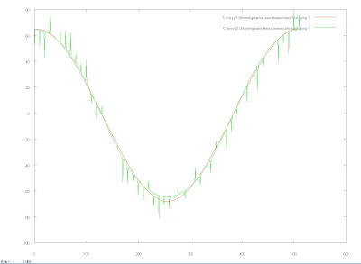
The following images show the ellipse projected onto the wavelets and then projected back to see how they compare to the data. The graph shows the data in red and the wavelet version in green, and as can be seen the data and wavelets show almost the exact same locations. The first graph is the ellipse points, the second the x points, and the third the y points.

One issue that came up was that the calculations on the wavelets came up with incorrect results when I used the program on a Linux machine. The code implements classes from the VNL library like vnl/algo/vnl_matrix_inverse and vnl/vnl_matrix to complete the computations. When run on a Linux machine the results showed that the wavelets version of the data were off at the edges and when I tried to transform the y points, it gave totally incorrect results like as follows with the data in green and the wavelet fit in red.

Cubic B-Spline Wavelets

The above is a graph of a few of the wavelets that are being used in the levels j = 0,...,2.

Point Representation Using Wavelets

The above graph represents all the points currently used at the start of the registration process. The points create an elliptical shape. To transform the points using wavelets, the x and y values were separated as shown in the following graphs.

Then Cubic B-Spline wavelets are created with j = 0,...,6, where j is the number of intervals. Scaling functions for j = 0 where also created. Then the scaling functions and wavelets were all put into a matrix by evaluating the function along the interval at 512 points for each wavelet or scaling function and storing those values along the rows. Then that matrix was multiplied by the actual function needing to be transformed, in this case the x or y values that made up 512 points, the result was a vector of coefficients that could be used to recreate the data by multiplying the scaling and wavelet matrix by the coefficient vector. The following graphs illustrate the results where the one on the left represents the x points and the one on the right represents the projection that resulted from the data being projected onto the wavelets.

The wavelet projection produces a set of points with a similar overall shape but the y axis is more then doubled in magnitude. This might be occurring because the wavelets need to be scaled.